Step 11: 2D Laplace Equation

---

Here is Laplace’s equation in 2D:

\[\frac{\partial ^2 p}{\partial x^2} + \frac{\partial ^2 p}{\partial y^2} = 0\]

We know how to discretize a 2nd order derivative. But think about this for a minute — Laplace’s equation has the features typical of diffusion phenomena. For this reason, it has to be discretized with central differences, so that the discretization is consistent with the physics we want to simulate.

The discretized equation is:

\[\frac{p_{i+1, j}^n - 2p_{i,j}^n + p_{i-1,j}^n}{\Delta x^2} + \frac{p_{i,j+1}^n - 2p_{i,j}^n + p_{i, j-1}^n}{\Delta y^2} = 0\]

Notice that the Laplace Equation does not have a time dependence — there is no \(p^{n+1}\). Instead of tracking a wave through time (like in the previous steps), the Laplace equation calculates the equilibrium state of a system under the supplied boundary conditions.

If you have taken coursework in Heat Transfer, you will recognize the Laplace Equation as the steady-state heat equation.

Instead of calculating where the system will be at some time \(t\), we will iteratively solve for \(p_{i,j}^n\) until it meets a condition that we specify. The system will reach equilibrium only as the number of iterations tends to \(\infty\), but we can approximate the equilibrium state by iterating until the change between one iteration and the next is very small.

Let’s rearrange the discretized equation, solving for \(p_{i,j}^n\):

\[p_{i,j}^n = \frac{\Delta y^2(p_{i+1,j}^n+p_{i-1,j}^n)+\Delta x^2(p_{i,j+1}^n + p_{i,j-1}^n)}{2(\Delta x^2 + \Delta y^2)}\]

Using second-order central-difference schemes in both directions is the most widely applied method for the Laplace operator. It is also known as the five-point difference operator.

We are going to solve Laplace’s equation numerically by assuming an initial state of \(p=0\) everywhere. Then we add boundary conditions as follows:

\(p=0\) at \(x=0\)

\(p=y\) at \(x=2\)

\(\frac{\partial p}{\partial y}=0\) at \(y=0, \ 1\)

Under these conditions, there is an analytical solution for Laplace’s equation:

\[p(x,y)=\frac{x}{4}-4\sum_{n=1,odd}^{\infty}\frac{1}{(n\pi)^2\sinh2n\pi}\sinh n\pi x\cos n\pi y\]

import numpy as np
from matplotlib import pyplot as plt, cm
from mpl_toolkits.mplot3d import Axes3D

def plot2D(x,y,p):  # define a function for visulizing 2d plot
    fig = plt.figure(figsize = (11,7), dpi=100)
    ax = fig.add_subplot(111, projection='3d')
    # The '111' means a grid of 1 row and 1 column and this subplot is the first one.
    X, Y = np.meshgrid(x,y)
    surf = ax.plot_surface(X,Y,p,cmap=cm.viridis)
    ax.set_xlabel('$x$')
    ax.set_ylabel('$y$');

\[p_{i,j}^n = \frac{\Delta y^2(p_{i+1,j}^n+p_{i-1,j}^n)+\Delta x^2(p_{i,j+1}^n + p_{i,j-1}^n)}{2(\Delta x^2 + \Delta y^2)}\]

def laplace2d(p, y, dx, dy, l1norm_target):
    l1norm = 1
    pn = np.zeros_like(p)
    
    while l1norm > l1norm_target:
        pn = p.copy()
        p[1:-1,1:-1] = ((dy**2 * (pn[2:,1:-1] + pn[:-2,1:-1]) +
                        dx**2 * (pn[1:-1,2:] + pn[1:-1,:-2])) /
                        (2 * (dx**2 + dy**2)))
        p[0,:] = 0  # p = 0 @ x = 0
        p[-1:,] = y # p = y @ x = 2
        p[:,0] = p[:,1] # dp/dy = 0 @ y = 0
        p[:,-1] = p[:,-2] # dp/dy = 0 @ y = 2  
        l1norm = (np.sum(np.abs(p[:])-np.abs(pn[:])) / np.sum(np.abs(pn[:])))
    return p

laplace2d takes five arguments, the p matrix, the y-vector, dx, dy and the value l1norm_target. This last value defines how close the p matrix should be in two consecutive iterations before the loop breaks and returns the calculated p value.

Note that when executing the cells above in your own notebook, there will be no output. You have defined the function but you have not yet called the function. It is now available for you to use, the same as numpy.linspace or any other function in our namespace.

##variable declarations
nx = 31
ny = 31
c = 1
dx = 2 / (nx - 1)
dy = 2 / (ny - 1)


##initial conditions
p = np.zeros((nx, ny))  # create a XxY vector of 0's


##plotting aids
x = np.linspace(0, 2, nx)
y = np.linspace(0, 1, ny)

##boundary conditions
p[:, 0] = 0  # p = 0 @ x = 0
p[:, -1] = y  # p = y @ x = 2
p[0, :] = p[1, :]  # dp/dy = 0 @ y = 0
p[-1, :] = p[-2, :]  # dp/dy = 0 @ y = 1

p_init = p.copy()

#hit the **tab** key for auto-complete options.  
plot2D(x,y,p_init)

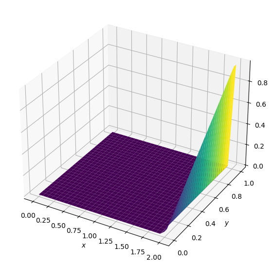
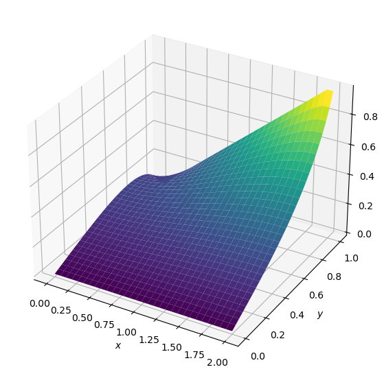
p = laplace2d(p, y, dx, dy, 1e-4)

It worked! This is the initial state of our problem, where the value of p is zero everywhere except for along \(x=2\) where \(p=y\). Now let’s try to run our laplace2d function with a specified L1 target of .01

[Hint: if you are having trouble remembering the order in which variables are sent to a function, you can just type laplace2d( and the iPython Notebook will put up a little popup box to remind you]

plot2D(x, y, p)