Step 4: Diffusion Equation in 1-D#
The one-dimensional diffusion equation is:
The first thing you should notice is that —unlike the previous two simple equations we have studied— this equation has a second-order derivative. We first need to learn what to do with it!
Discretizing \(\frac{\partial ^2 u}{\partial x^2}\)#
The second-order derivative can be represented geometrically as the line tangent to the curve given by the first derivative. We will discretize the second-order derivative with a Central Difference scheme: a combination of Forward Difference and Backward Difference of the first derivative. Consider the Taylor expansion of \(u_{i+1}\) and \(u_{i-1}\) around \(u_i\):
\(u_{i+1} = u_i + \Delta x \frac{\partial u}{\partial x}\bigg|_i + \frac{\Delta x^2}{2} \frac{\partial ^2 u}{\partial x^2}\bigg|_i + \frac{\Delta x^3}{3!} \frac{\partial ^3 u}{\partial x^3}\bigg|_i + O(\Delta x^4)\)
\(u_{i-1} = u_i - \Delta x \frac{\partial u}{\partial x}\bigg|_i + \frac{\Delta x^2}{2} \frac{\partial ^2 u}{\partial x^2}\bigg|_i - \frac{\Delta x^3}{3!} \frac{\partial ^3 u}{\partial x^3}\bigg|_i + O(\Delta x^4)\)
If we add these two expansions, you can see that the odd-numbered derivative terms will cancel each other out. If we neglect any terms of \(O(\Delta x^4)\) or higher (and really, those are very small), then we can rearrange the sum of these two expansions to solve for our second-derivative.
\(u_{i+1} + u_{i-1} = 2u_i+\Delta x^2 \frac{\partial ^2 u}{\partial x^2}\bigg|_i + O(\Delta x^4)\)
Then rearrange to solve for \(\frac{\partial ^2 u}{\partial x^2}\bigg|_i\) and the result is:
Back to Step 4#
We can now write the discretized version of the diffusion equation in 1D:
As before, we notice that once we have an initial condition, the only unknown is \(u_{i}^{n+1}\), so we re-arrange the equation solving for our unknown:
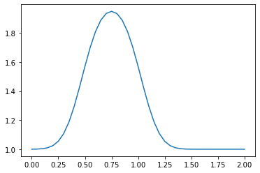
The above discrete equation allows us to write a program to advance a solution in time. But we need an initial condition. Let’s continue using our favorite: the hat function. So, at \(t=0\), \(u=2\) in the interval \(0.5\le x\le 1\) and \(u=1\) everywhere else. We are ready to go!
import numpy as np
from matplotlib import pyplot as plt
nx = 41
dx = 2 / (nx - 1)
nt = 20 # the number of timesteps
nu = 0.3 # diffusion coefficient
sigma = 0.2 # sigma is a numerical parameter, we will learn it later
dt = sigma * dx**2 / nu  # dt is defined using sigma

u = np.ones(nx) # a numpy array with nx elements all equal to 1
u[int(0.5/dx):int(1/dx+1)] = 2 # setting u = 2 between 0.5 and 1

un = np.ones(nx) # our placeholder array to advance the solution in time

for n in range(nt): # iterate through 0 to nt-1, in total nt steps
    un = u.copy() # copy the existing values of u into un
    for i in range(1, nx-1): # skip first and last component!
        u[i] = un[i] + nu * dt / dx**2 * (un[i+1] - 2 * un[i] + un[i-1])

plt.plot(np.linspace(0,2,nx),u)
[<matplotlib.lines.Line2D at 0x7f27c8150550>]