The the next steps in this interactive module will both solve the Navier–Stokes equations in two dimensions, but with different boundary conditions.
The momentum equation in vector form for a velocity field \(\vec{v}\) is:
This represents three scalar equations, one for each velocity component \((u,v,w)\). But we will solve it in two dimensions, so there will be two scalar equations.
Remember the continuity equation? $\( \begin{eqnarray*} \nabla \cdot\vec{v} &=& 0 \end{eqnarray*} \)$ This is where the [Poisson equation] for pressure comes in!
Step 13.1: Cavity Flow with Navier–Stokes#
Here is the system of differential equations: two equations for the velocity components \(u,v\) and one equation for pressure:
Discretized equations#
First, let’s discretize the \(u\)-momentum equation, as follows: $\( \begin{split} & \frac{u_{i,j}^{n+1}-u_{i,j}^{n}}{\Delta t}+u_{i,j}^{n}\frac{u_{i,j}^{n}-u_{i-1,j}^{n}}{\Delta x}+v_{i,j}^{n}\frac{u_{i,j}^{n}-u_{i,j-1}^{n}}{\Delta y} = \\ & \qquad -\frac{1}{\rho}\frac{p_{i+1,j}^{n}-p_{i-1,j}^{n}}{2\Delta x}+\nu\left(\frac{u_{i+1,j}^{n}-2u_{i,j}^{n}+u_{i-1,j}^{n}}{\Delta x^2}+\frac{u_{i,j+1}^{n}-2u_{i,j}^{n}+u_{i,j-1}^{n}}{\Delta y^2}\right) \end{split} \)$
Similarly for the \(v\)-momentum equation: $\( \begin{split} &\frac{v_{i,j}^{n+1}-v_{i,j}^{n}}{\Delta t}+u_{i,j}^{n}\frac{v_{i,j}^{n}-v_{i-1,j}^{n}}{\Delta x}+v_{i,j}^{n}\frac{v_{i,j}^{n}-v_{i,j-1}^{n}}{\Delta y} = \\ & \qquad -\frac{1}{\rho}\frac{p_{i,j+1}^{n}-p_{i,j-1}^{n}}{2\Delta y} +\nu\left(\frac{v_{i+1,j}^{n}-2v_{i,j}^{n}+v_{i-1,j}^{n}}{\Delta x^2}+\frac{v_{i,j+1}^{n}-2v_{i,j}^{n}+v_{i,j-1}^{n}}{\Delta y^2}\right) \end{split} \)$
Finally, the discretized pressure-Poisson equation can be written thus: : $\( \begin{split} & \frac{p_{i+1,j}^{n}-2p_{i,j}^{n}+p_{i-1,j}^{n}}{\Delta x^2}+\frac{p_{i,j+1}^{n}-2p_{i,j}^{n}+p_{i,j-1}^{n}}{\Delta y^2} = \\ & \qquad \rho \left[ \frac{1}{\Delta t}\left(\frac{u_{i+1,j}-u_{i-1,j}}{2\Delta x}+\frac{v_{i,j+1}-v_{i,j-1}}{2\Delta y}\right) -\frac{u_{i+1,j}-u_{i-1,j}}{2\Delta x}\frac{u_{i+1,j}-u_{i-1,j}}{2\Delta x} - 2\frac{u_{i,j+1}-u_{i,j-1}}{2\Delta y}\frac{v_{i+1,j}-v_{i-1,j}}{2\Delta x} - \frac{v_{i,j+1}-v_{i,j-1}}{2\Delta y}\frac{v_{i,j+1}-v_{i,j-1}}{2\Delta y}\right] \end{split} \)$
You should write these equations down on your own notes, by hand, following each term mentally as you write it.
As before, let’s rearrange the equations in the way that the iterations need to proceed in the code. First, the momentum equations for the velocity at the next time step.
The momentum equation in the \(u\) direction:
The momentum equation in the \(v\) direction:
Almost there! Now, we rearrange the pressure-Poisson equation:
The initial condition is \(u, v, p = 0\) everywhere, and the boundary conditions are:
\(u=1\) at \(y=2\) (the “lid”);
\(u, v=0\) on the other boundaries;
\(\frac{\partial p}{\partial y}=0\) at \(y=0\);
\(p=0\) at \(y=2\)
\(\frac{\partial p}{\partial x}=0\) at \(x=0,2\)
import numpy as np
from matplotlib import pyplot as plt, cm
from mpl_toolkits.mplot3d import Axes3D
nx = 41
ny = 41
nt = 500
nit = 50
c = 1
length = 1
dx = length / (nx-1)
dy = length / (ny-1)
x = np.linspace(0,length,nx)
y = np.linspace(0,length,ny)
X, Y = np.meshgrid(x, y)

rho = 1
nu = 0.01
dt = 0.001

u = np.zeros((ny,nx))
v = np.zeros((ny,nx))
p = np.zeros((ny,nx))
b = np.zeros((ny,nx))

print("Reynold's number =", c*length/nu)
Reynold's number = 100.0
The pressure Poisson equation that’s written above can be hard to write out without typos. The function build_up_b below represents the contents of the square brackets, so that the entirety of the PPE is slightly more manageable.
$\(\frac{\partial^2 p}{\partial x^2}+\frac{\partial^2 p}{\partial y^2} = \rho\left(\frac{\partial}{\partial t}\left(\frac{\partial u}{\partial x} +\frac{\partial v}{\partial y} \right) - \frac{\partial u}{\partial x}\frac{\partial u}{\partial x}-2\frac{\partial u}{\partial y}\frac{\partial v}{\partial x}-\frac{\partial v}{\partial y}\frac{\partial v}{\partial y} \right)\)$
def build_up_b(b, rho, dt, u, v, dx, dy):

    b[1:-1, 1:-1] = (rho * (1 / dt *
                    ((u[1:-1, 2:] - u[1:-1, 0:-2]) /
                     (2 * dx) + (v[2:, 1:-1] - v[0:-2, 1:-1]) / (2 * dy)) -
                    ((u[1:-1, 2:] - u[1:-1, 0:-2]) / (2 * dx))**2 -
                      2 * ((u[2:, 1:-1] - u[0:-2, 1:-1]) / (2 * dy) *
                           (v[1:-1, 2:] - v[1:-1, 0:-2]) / (2 * dx))-
                          ((v[2:, 1:-1] - v[0:-2, 1:-1]) / (2 * dy))**2))


    return b
The function pressure_poisson is also defined to help segregate the different rounds of calculations. Note the presence of the pseudo-time variable nit. This sub-iteration in the Poisson calculation helps ensure a divergence-free field.
def pressure_poisson(p, dx, dy, b):
    pn = np.empty_like(p)
    pn = p.copy()

    for q in range(nit):
        pn = p.copy()
        p[1:-1, 1:-1] = (((pn[1:-1, 2:] + pn[1:-1, 0:-2]) * dy**2 +
                          (pn[2:, 1:-1] + pn[0:-2, 1:-1]) * dx**2) /
                          (2 * (dx**2 + dy**2)) -
                          dx**2 * dy**2 / (2 * (dx**2 + dy**2)) *
                          b[1:-1,1:-1])

        p[:, -1] = p[:, -2] # dp/dx = 0 at x = 2
        p[0, :] = p[1, :]   # dp/dy = 0 at y = 0
        p[:, 0] = p[:, 1]   # dp/dx = 0 at x = 0
        p[-1, :] = 0        # p = 0 at y = 2

    return p
# This is another version of pressure_poisson function with l1norm_target
def pressure_poisson_l1norm(p, dx, dy, b, l1norm_target):
    pn = np.empty_like(p)
    pn = p.copy()

    l1norm = 1
    small = 1e-8
    niter = 0
    while l1norm > l1norm_target:
        niter += 1   # count the number of iterations for convergence
        pn = p.copy()
        p[1:-1, 1:-1] = (((pn[1:-1, 2:] + pn[1:-1, 0:-2]) * dy**2 +
                          (pn[2:, 1:-1] + pn[0:-2, 1:-1]) * dx**2) /
                          (2 * (dx**2 + dy**2)) -
                          dx**2 * dy**2 / (2 * (dx**2 + dy**2)) *
                          b[1:-1,1:-1])

        p[:, -1] = p[:, -2] # dp/dx = 0 at x = 2
        p[0, :] = p[1, :]   # dp/dy = 0 at y = 0
        p[:, 0] = p[:, 1]   # dp/dx = 0 at x = 0
        p[-1, :] = 0        # p = 0 at y = 2
        l1norm = (np.sum(np.abs(p[:]-pn[:])) / (np.sum(np.abs(pn[:]))+small))

    return p, niter
The momentum equation in the \(u\) direction:
The momentum equation in the \(v\) direction:
def velocity_u_update(u, dx, dy, dt, rho, p, un, vn):

    u[1:-1, 1:-1] = (un[1:-1, 1:-1]-
                    un[1:-1, 1:-1] * dt / dx *
                    (un[1:-1, 1:-1] - un[1:-1, 0:-2]) -
                    vn[1:-1, 1:-1] * dt / dy *
                    (un[1:-1, 1:-1] - un[0:-2, 1:-1]) -
                    dt / (2 * rho * dx) * (p[1:-1, 2:] - p[1:-1, 0:-2]) +
                    nu * (dt / dx**2 *
                    (un[1:-1, 2:] - 2 * un[1:-1, 1:-1] + un[1:-1, 0:-2]) +
                    dt / dy**2 *
                    (un[2:, 1:-1] - 2 * un[1:-1, 1:-1] + un[0:-2, 1:-1])))
    return u

def velocity_v_update(v, dx, dy, dt, rho, p, un, vn):

    v[1:-1,1:-1] = (vn[1:-1, 1:-1] -
                    un[1:-1, 1:-1] * dt / dx *
                    (vn[1:-1, 1:-1] - vn[1:-1, 0:-2]) -
                    vn[1:-1, 1:-1] * dt / dy *
                    (vn[1:-1, 1:-1] - vn[0:-2, 1:-1]) -
                    dt / (2 * rho * dy) * (p[2:, 1:-1] - p[0:-2, 1:-1]) +
                    nu * (dt / dx**2 *
                    (vn[1:-1, 2:] - 2 * vn[1:-1, 1:-1] + vn[1:-1, 0:-2]) +
                    dt / dy**2 *
                    (vn[2:, 1:-1] - 2 * vn[1:-1, 1:-1] + vn[0:-2, 1:-1])))
    return v
Finally, the rest of the cavity flow equations are wrapped inside the function cavity_flow, allowing us to easily plot the results of the cavity flow solver for different lengths of time.
def cavity_flow(nt, u, v, dt, dx, dy, p, rho, nu):
    un = np.empty_like(u)
    vn = np.empty_like(v)
    pn = np.empty_like(p)
    b = np.zeros((ny, nx))
    small = 1e-8
    for n in range(nt):
        un = u.copy()
        vn = v.copy()
        pn = p.copy()
        b = build_up_b(b, rho, dt, u, v, dx, dy)
        #p = pressure_poisson(p, dx, dy, b)
        p, niter = pressure_poisson_l1norm(p, dx, dy, b, 1e-4)
        #print(niter)

        u = velocity_u_update(u, dx, dy, dt, rho, p, un, vn)
        v = velocity_v_update(v, dx, dy, dt, rho, p, un, vn)

        u[0, :]  = 0
        u[:, 0]  = 0
        u[:, -1] = 0
        u[-1, :] = c    # set velocity on cavity lid equal to c
        v[0, :]  = 0
        v[-1, :] = 0
        v[:, 0]  = 0
        v[:, -1] = 0

    l1norm_u = (np.sum(np.abs(u[:]-un[:])) / (np.sum(np.abs(un[:]))+small))
    l1norm_v = (np.sum(np.abs(v[:]-vn[:])) / (np.sum(np.abs(vn[:]))+small))
    l1norm_p = (np.sum(np.abs(p[:]-pn[:])) / (np.sum(np.abs(pn[:]))+small))
    print("l1norm_u = ",  l1norm_u, "l1norm_v = ",  l1norm_v, "l1norm_p = ",  l1norm_p)
    return u, v, p
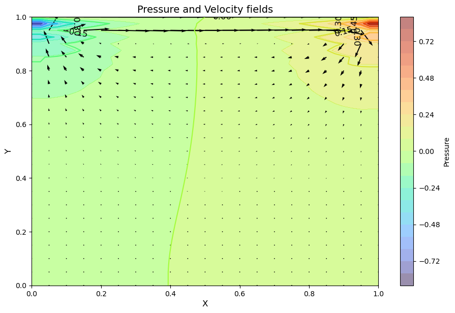
Let’s start with nt = 100 and see what the solver gives us:
u = np.zeros((ny, nx))
v = np.zeros((ny, nx))
p = np.zeros((ny, nx))
b = np.zeros((ny, nx))
nt = 100
u, v, p = cavity_flow(nt, u, v, dt, dx, dy, p, rho, nu)
l1norm_u = 0.0037345482982977384 l1norm_v = 0.01107964897409599 l1norm_p = 0.001136767295111687
# Create figure and set dpi and figure size
fig = plt.figure(figsize=(11,7), dpi=100)

# Contourf plot for pressure field with colorbar
cf = plt.contourf(X, Y, p, alpha=0.5, cmap='turbo', levels=20)
plt.colorbar(cf, label='Pressure')

# Contour plot for pressure field outlines
contour = plt.contour(X, Y, p, cmap='turbo', levels=10)
plt.clabel(contour, inline=False, fontsize=12, colors = 'black')

# Quiver plot for velocity field
quiv = plt.quiver(X[::2, ::2], Y[::2, ::2], u[::2, ::2], v[::2, ::2])

# Setting labels for the x and y axes
plt.xlabel('X', fontsize=12)
plt.ylabel('Y', fontsize=12)

# Setting the title for the plot
plt.title('Pressure and Velocity fields', fontsize=14)

# Display the plot
plt.show()
#%%timeit -r 1 -n 1
u = np.zeros((ny, nx))
v = np.zeros((ny, nx))
p = np.zeros((ny, nx))
b = np.zeros((ny, nx))
nt = 10000
u, v, p = cavity_flow(nt, u, v, dt, dx, dy, p, rho, nu)
l1norm_u = 2.0964336749894792e-06 l1norm_v = 2.8019156614369277e-06 l1norm_p = 2.349586199251818e-06
# Create figure and set dpi and figure size
fig = plt.figure(figsize=(11,7), dpi=100)

# Contourf plot for pressure field with colorbar
cf = plt.contourf(X, Y, p, alpha=0.5, cmap='turbo', levels=20)
plt.colorbar(cf, label='Pressure')

# Contour plot for pressure field outlines
contour = plt.contour(X, Y, p, cmap='turbo', levels=10)
plt.clabel(contour, inline=False, fontsize=12, colors = 'black')

# Quiver plot for velocity field
quiv = plt.quiver(X[::2, ::2], Y[::2, ::2], u[::2, ::2], v[::2, ::2])

# Setting labels for the x and y axes
plt.xlabel('X', fontsize=12)
plt.ylabel('Y', fontsize=12)

# Setting the title for the plot
plt.title('Pressure and Velocity fields', fontsize=14)

# Display the plot
plt.show()
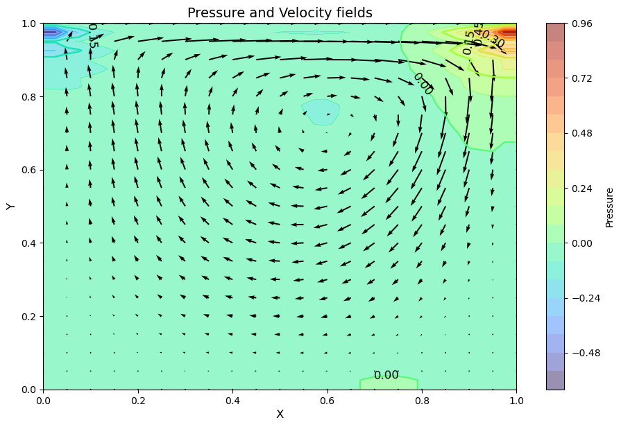
The quiver plot shows the magnitude of the velocity at the discrete points in the mesh grid we created.
(We’re actually only showing half of the points because otherwise it’s a bit of a mess. The X[::2, ::2] syntax above is a convenient way to ask for every other point.)
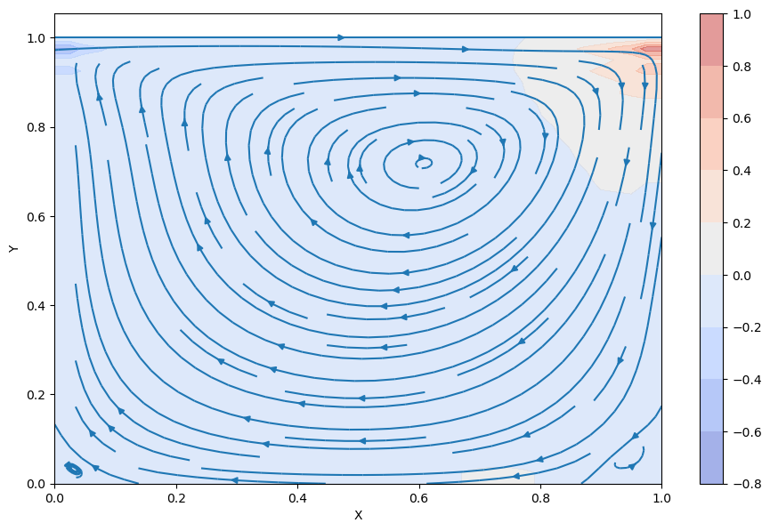
Another way to visualize the flow in the cavity is to use a streamplot:
fig = plt.figure(figsize=(11, 7), dpi=100)
plt.contourf(X, Y, p, alpha=0.5, cmap=cm.coolwarm)
plt.colorbar()
#plt.contour(X, Y, p, cmap=cm.coolwarm)
plt.streamplot(X, Y, u, v)
plt.xlabel('X')
plt.ylabel('Y');
Benchmark using a reference data (Ghia-1982)#
import pandas as pd
import matplotlib.pyplot as plt
# Read the txt file
with open('Ghia-1982.txt', 'r') as file:
lines = file.readlines()
# Adjust the lines range to match your data
lines = lines[5:-7] # Adjust these numbers
# Process lines to obtain data
data = [list(map(float, line.split())) for line in lines]
# Create DataFrame from data
df = pd.DataFrame(data, columns=['y', 'Re=100', 'Re=400', 'Re=1000', 'Re=3200', 'Re=5000', 'Re=7500', 'Re=10000'])
# Set y as index
df.set_index('y', inplace=True)
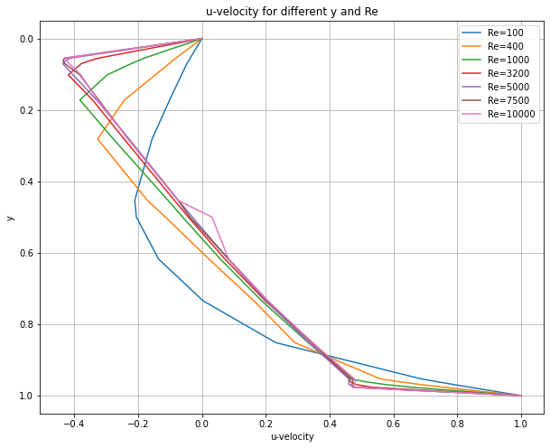
# Plotting
plt.figure(figsize=(10,8))
for column in df.columns:
plt.plot(df[column].values, df.index.values, label=column) # use .values to get numpy arrays
plt.xlabel('u-velocity')
plt.ylabel('y')
plt.title('u-velocity for different y and Re')
plt.legend()
plt.gca().invert_yaxis() # To invert y-axis
plt.grid(True)
plt.show()
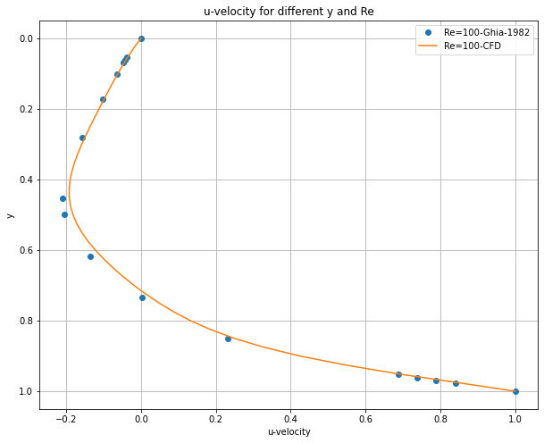
# Plotting
plt.figure(figsize=(10,8))

plt.plot(df['Re=100'].values, df.index.values, 'o', label='Re=100-Ghia-1982') # use .values to get numpy arrays
plt.plot(u[:,int(ny/2)], y, label='Re=100-CFD') #

plt.xlabel('u-velocity')
plt.ylabel('y')
plt.title('u-velocity for different y and Re')
plt.legend()
plt.gca().invert_yaxis()  # To invert y-axis
plt.grid(True)
plt.show()
Try a case with Re = 400 and what happens?#
rho = 1
c= 2.5
nu = 0.01
dt = 0.001

u = np.zeros((ny,nx))
v = np.zeros((ny,nx))
p = np.zeros((ny,nx))
b = np.zeros((ny,nx))

print("Reynold's number =", c*length/nu)
Reynold's number = 250.0
nt = 10000
u, v, p = cavity_flow(nt, u, v, dt, dx, dy, p, rho, nu)

# Create figure and set dpi and figure size
fig = plt.figure(figsize=(11,7), dpi=100)

# Contourf plot for pressure field with colorbar
cf = plt.contourf(X, Y, p, alpha=0.5, cmap='turbo', levels=20)
plt.colorbar(cf, label='Pressure')

# Contour plot for pressure field outlines
contour = plt.contour(X, Y, p, cmap='turbo', levels=10)
plt.clabel(contour, inline=False, fontsize=12, colors = 'black')

# Quiver plot for velocity field
quiv = plt.quiver(X[::2, ::2], Y[::2, ::2], u[::2, ::2], v[::2, ::2])

# Setting labels for the x and y axes
plt.xlabel('X', fontsize=12)
plt.ylabel('Y', fontsize=12)

# Setting the title for the plot
plt.title('Pressure and Velocity fields', fontsize=14)

# Display the plot
plt.show()
/tmp/ipykernel_22183/2990769937.py:6: RuntimeWarning: overflow encountered in square
  ((u[1:-1, 2:] - u[1:-1, 0:-2]) / (2 * dx))**2 -
/tmp/ipykernel_22183/2990769937.py:7: RuntimeWarning: overflow encountered in multiply
  2 * ((u[2:, 1:-1] - u[0:-2, 1:-1]) / (2 * dy) *
/tmp/ipykernel_22183/2990769937.py:7: RuntimeWarning: overflow encountered in divide
  2 * ((u[2:, 1:-1] - u[0:-2, 1:-1]) / (2 * dy) *
/tmp/ipykernel_22183/2990769937.py:3: RuntimeWarning: invalid value encountered in subtract
  b[1:-1, 1:-1] = (rho * (1 / dt *
/tmp/ipykernel_22183/2990769937.py:9: RuntimeWarning: overflow encountered in square
  ((v[2:, 1:-1] - v[0:-2, 1:-1]) / (2 * dy))**2))
/tmp/ipykernel_22183/1422217961.py:4: RuntimeWarning: overflow encountered in multiply
  un[1:-1, 1:-1] * dt / dx *
/tmp/ipykernel_22183/1422217961.py:6: RuntimeWarning: overflow encountered in multiply
  vn[1:-1, 1:-1] * dt / dy *
/tmp/ipykernel_22183/1422217961.py:8: RuntimeWarning: invalid value encountered in subtract
  dt / (2 * rho * dx) * (p[1:-1, 2:] - p[1:-1, 0:-2]) +
/tmp/ipykernel_22183/1422217961.py:18: RuntimeWarning: overflow encountered in multiply
  un[1:-1, 1:-1] * dt / dx *
/tmp/ipykernel_22183/1422217961.py:20: RuntimeWarning: overflow encountered in multiply
  vn[1:-1, 1:-1] * dt / dy *
/tmp/ipykernel_22183/1422217961.py:17: RuntimeWarning: overflow encountered in subtract
  v[1:-1,1:-1] = (vn[1:-1, 1:-1] -
/tmp/ipykernel_22183/1422217961.py:17: RuntimeWarning: invalid value encountered in subtract
  v[1:-1,1:-1] = (vn[1:-1, 1:-1] -
/tmp/ipykernel_22183/1422217961.py:22: RuntimeWarning: invalid value encountered in subtract
  dt / (2 * rho * dy) * (p[2:, 1:-1] - p[0:-2, 1:-1]) +
/tmp/ipykernel_22183/1422217961.py:19: RuntimeWarning: invalid value encountered in subtract
  (vn[1:-1, 1:-1] - vn[1:-1, 0:-2]) -
/tmp/ipykernel_22183/1422217961.py:24: RuntimeWarning: invalid value encountered in subtract
  (vn[1:-1, 2:] - 2 * vn[1:-1, 1:-1] + vn[1:-1, 0:-2]) +
l1norm_u = nan l1norm_v = nan l1norm_p = nan
/tmp/ipykernel_22183/2565152488.py:12: UserWarning: No contour levels were found within the data range.
  contour = plt.contour(X, Y, p, cmap='turbo', levels=10)
What happened?#
We employed the backward differencing scheme for the convection term. Theoretically, this approach is apt for positive velocities. However, when the Reynolds number is high, leading to significantly negative velocities, the results tend to be unstable. As a next step, we will implement the upwind scheme for the convection term to assess its performance under high Reynolds number scenarios.