Step 7: 2D Linear Convection

---

Up to now, all of our work has been in one spatial dimension. We can learn a lot in just 1D, but let’s grow up to flatland: two dimensions.

In the following exercises, you will extend the first four steps to 2D. To extend the 1D finite-difference formulas to partial derivatives in 2D or 3D, just apply the definition: a partial derivative with respect to \(x\) is the variation in the \(x\) direction at constant \(y\).

In 2D space, a rectangular (uniform) grid is defined by the points with coordinates:

\[x_i = x_0 +i \Delta x\]

\[y_i = y_0 +i \Delta y\]

Now, define \(u_{i,j} = u(x_i,y_j)\) and apply the finite-difference formulas on either variable \(x,y\) acting separately on the \(i\) and \(j\) indices. All derivatives are based on the 2D Taylor expansion of a mesh point value around \(u_{i,j}\).

Hence, for a first-order partial derivative in the \(x\)-direction, a finite-difference formula is:

\[ \frac{\partial u}{\partial x}\biggr\rvert_{i,j} = \frac{u_{i+1,j}-u_{i,j}}{\Delta x}+\mathcal{O}(\Delta x)\]

and similarly in the \(y\) direction. Thus, we can write backward-difference, forward-difference or central-difference formulas. Let’s get started!

The PDE governing 2-D Linear Convection is written as

\[\frac{\partial u}{\partial t}+c\frac{\partial u}{\partial x} + c\frac{\partial u}{\partial y} = 0\]

This is the exact same form as with 1-D Linear Convection, except that we now have two spatial dimensions to account for as we step forward in time.

Again, the timestep will be discretized as a forward difference and both spatial steps will be discretized as backward differences.

With 1-D implementations, we used \(i\) subscripts to denote movement in space (e.g. \(u_{i}^n-u_{i-1}^n\)). Now that we have two dimensions to account for, we need to add a second subscript, \(j\), to account for all the information in the regime.

Here, we’ll again use \(i\) as the index for our \(x\) values, and we’ll add the \(j\) subscript to track our \(y\) values.

With that in mind, our discretization of the PDE should be relatively straightforward.

\[\frac{u_{i,j}^{n+1}-u_{i,j}^n}{\Delta t} + c\frac{u_{i, j}^n-u_{i-1,j}^n}{\Delta x} + c\frac{u_{i,j}^n-u_{i,j-1}^n}{\Delta y}=0\]

As before, solve for the only unknown:

\[u_{i,j}^{n+1} = u_{i,j}^n-c \frac{\Delta t}{\Delta x}(u_{i,j}^n-u_{i-1,j}^n)-c \frac{\Delta t}{\Delta y}(u_{i,j}^n-u_{i,j-1}^n)\]

We will solve this equation with the following initial conditions:

\[u(x,y) = \begin{cases} \begin{matrix} 2\ \text{for} & 0.5 \leq x, y \leq 1 \cr 1\ \text{for} & \text{everywhere else}\end{matrix}\end{cases}\]

and boundary conditions:

\[u = 1\ \text{for } \begin{cases} \begin{matrix} x = 0,\ 2 \cr y = 0,\ 2 \end{matrix}\end{cases}\]

from mpl_toolkits.mplot3d import Axes3D #New library required for projected 3d plots
import numpy as np
from matplotlib import pyplot as plt, cm

#variables declarations

nx = 81
ny = 81
nt = 100
c = 1

dx = 2 / (nx - 1)
dy = 2 / (ny - 1)
sigma =.2
dt = sigma * dx

x = np.linspace(0,2,nx)
y = np.linspace(0,2,nx)

u = np.ones((nx,ny)) # create 2d array of 1's
un = np.ones((nx,ny)) # placeholder

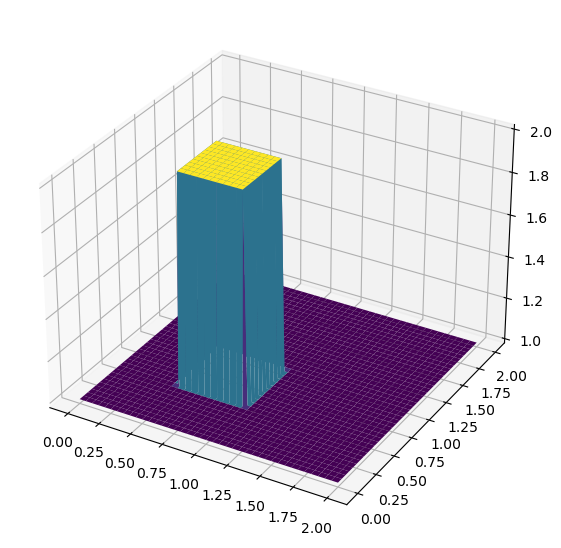
## inital conditions

# set hat function I.C.: u(0.5<=x<=1 && 0.5<=y<=1) = 2
u[int(0.5/dx):int(1/dx + 1),int(0.5/dy):int(1/dy + 1)] = 2

#plot initical condition
fig = plt.figure(figsize = (11,7), dpi=100)
ax = fig.add_subplot(111, projection='3d')
# The '111' means a grid of 1 row and 1 column and this subplot is the first one.
X, Y = np.meshgrid(x,y)
surf = ax.plot_surface(X,Y,u,cmap=cm.viridis)

Iterating in two dimensions

To evaluate the wave in two dimensions requires the use of several nested for-loops to cover all of the i’s and j’s. Since Python is not a compiled language there can be noticeable slowdowns in the execution of code with multiple for-loops. First try evaluating the 2D convection code and see what results it produces. $\(u_{i,j}^{n+1} = u_{i,j}^n-c \frac{\Delta t}{\Delta x}(u_{i,j}^n-u_{i-1,j}^n)-c \frac{\Delta t}{\Delta y}(u_{i,j}^n-u_{i,j-1}^n)\)$

%%timeit
u = np.ones((nx,ny))
u[int(0.5/dx):int(1/dx + 1),int(0.5/dy):int(1/dy + 1)] = 2

#loop across number of time steps
for n in range(nt):
    un = u.copy()
    row, col = u.shape
    for i in range(1,row):
        for j in range(1,col):
            u[i,j] = (un[i,j] - (c * dt / dx * (un[i,j] - un[i-1,j])) -
                                (c * dt / dy * (un[i,j] - un[i,j-1])))
            u[0,:] = 1
            u[:,0] = 1

768 ms ± 4.12 ms per loop (mean ± std. dev. of 7 runs, 1 loop each)

Here’s a detailed explanation of the %%timeit magic command:

Temporary Execution: The %%timeit magic command executes the code in a separate scope or context. It runs the code several times (for timing and averaging purposes) in a temporary context. Any changes made to variables, including arrays, within the %%timeit block do not affect the variables in the main environment.

No Permanent Changes: Since %%timeit is designed for measuring performance and not for making permanent changes to variables or data structures, any update or modification to an array inside a %%timeit cell is not reflected outside that cell.

Array Unchanged: As a result, when you update an array within a %%timeit cell and then try to view the array outside of this cell, you’ll see the original, unchanged array. The updates you made inside %%timeit do not persist.

To observe the changes you’ve made to an array, you need to update the array outside of the %%timeit cell. You can then use %%timeit separately to measure the performance of the update operation without expecting it to modify the array for later use.

u = np.ones((nx,ny))
u[int(0.5/dx):int(1/dx + 1),int(0.5/dy):int(1/dy + 1)] = 2

#loop across number of time steps
for n in range(nt):
    un = u.copy()
    row, col = u.shape
    for i in range(1,row):
        for j in range(1,col):
            u[i,j] = (un[i,j] - (c * dt / dx * (un[i,j] - un[i-1,j])) -
                                (c * dt / dy * (un[i,j] - un[i,j-1])))
            u[0,:] = 1
            u[:,0] = 1

fig = plt.figure(figsize = (11,7), dpi=100)
ax = fig.add_subplot(111, projection='3d')
# The '111' means a grid of 1 row and 1 column and this subplot is the first one.
X, Y = np.meshgrid(x,y)
surf = ax.plot_surface(X,Y,u,cmap=cm.viridis)

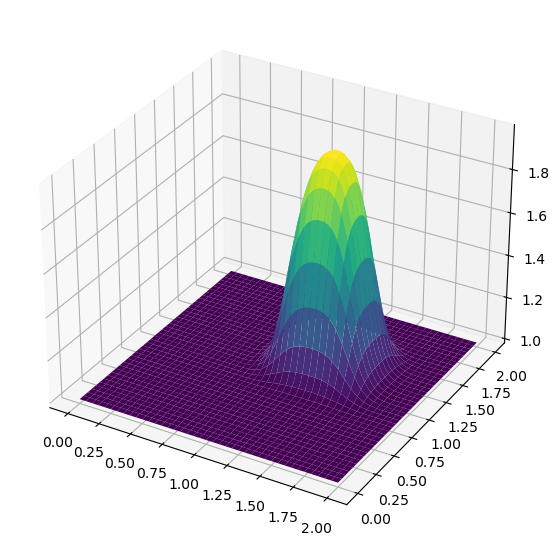
Array Operations

Here the same 2D convection code is implemented, but instead of using nested for-loops, the same calculations are evaluated using array operations.

%%timeit
u = np.ones((nx,ny))
u[int(0.5/dx):int(1/dx + 1),int(0.5/dy):int(1/dy + 1)] = 2

# loop across number of time steps
for n in range(nt):
    un = u.copy()
    u[1:,1:] = (un[1:,1:] - (c * dt / dx * (un[1:,1:] - un[:-1,1:])) -
                            (c * dt / dy * (un[1:,1:] - un[1:,:-1])))
    u[0,:] = 1
    u[:,0] = 1
    

2.63 ms ± 153 µs per loop (mean ± std. dev. of 7 runs, 100 loops each)

u = np.ones((nx,ny))
u[int(0.5/dx):int(1/dx + 1),int(0.5/dy):int(1/dy + 1)] = 2

# loop across number of time steps
for n in range(nt):
    un = u.copy()
    u[1:,1:] = (un[1:,1:] - (c * dt / dx * (un[1:,1:] - un[:-1,1:])) -
                            (c * dt / dy * (un[1:,1:] - un[1:,:-1])))
    u[0,:] = 1
    u[:,0] = 1


fig = plt.figure(figsize = (11,7), dpi=100)
ax = fig.add_subplot(111, projection='3d')
# The '111' means a grid of 1 row and 1 column and this subplot is the first one.
X, Y = np.meshgrid(x,y)
surf = ax.plot_surface(X,Y,u,cmap=cm.viridis)    

It’s evident that the array operations approach significantly outperforms the for-loop method in terms of speed and efficiency!