Step 13.3: Cavity flow with Chorin’s Projection#
Solution strategy: (Projection Method: Chorin’s Splitting)
https://www.youtube.com/watch?v=BQLvNLgMTQE&t=106s
Solve Momentum equation without pressure gradient for tentative velocity (with given Boundary Conditions)
Solve pressure poisson equation for pressure at next point in time (with homogeneous Neumann Boundary Conditions everywhere except for the top, where it is homogeneous Dirichlet)
Correct the velocities (and again enforce the Velocity Boundary Conditions)
The initial condition is \(u, v, p = 0\) everywhere, and the boundary conditions are:
\(u=1\) at \(y=2\) (the “lid”);
\(u, v=0\) on the other boundaries;
\(\frac{\partial p}{\partial y}=0\) at \(y=0\);
\(p=0\) at \(y=2\)
\(\frac{\partial p}{\partial x}=0\) at \(x=0,2\)
import numpy as np
from matplotlib import pyplot as plt, cm
from mpl_toolkits.mplot3d import Axes3D
from tqdm import tqdm
import time
#The tqdm library provides a progress bar for loops.
nx = 41
ny = 41
nt = 500
nit = 50
c = 1
length = 1
dx = length / (nx-1)
dy = length / (ny-1)
x = np.linspace(0,length,nx)
y = np.linspace(0,length,ny)
X, Y = np.meshgrid(x, y)

rho = 1
nu = 0.01
dt = 0.001

u = np.zeros((ny,nx))
v = np.zeros((ny,nx))
p = np.zeros((ny,nx))
b = np.zeros((ny,nx))

print("Reynold's number =", c*length/nu)

maximum_possible_time_step_length = 0.5 * dx**2 / nu
if dt > maximum_possible_time_step_length:
        print("Stability is not guarenteed")
Reynold's number = 100.0
def velocity_u_update(u, dx, dy, dt, rho, p, un, vn):  # Central differencing for convection term

    u[1:-1, 1:-1] = (un[1:-1, 1:-1]-
                    un[1:-1, 1:-1] * dt / (2*dx) *
                    (un[1:-1, 2:] - un[1:-1, 0:-2]) -
                    vn[1:-1, 1:-1] * dt / (2*dy) *
                    (un[2:, 1:-1] - un[0:-2, 1:-1]) +
                    nu * (dt / dx**2 *
                    (un[1:-1, 2:] - 2 * un[1:-1, 1:-1] + un[1:-1, 0:-2]) +
                    dt / dy**2 *
                    (un[2:, 1:-1] - 2 * un[1:-1, 1:-1] + un[0:-2, 1:-1])))
    return u

def velocity_v_update(v, dx, dy, dt, rho, p, un, vn): # Central differencing for convection term

    v[1:-1,1:-1] = (vn[1:-1, 1:-1] -
                    un[1:-1, 1:-1] * dt / (2*dx) *
                    (vn[1:-1, 2:] - vn[1:-1, 0:-2]) -
                    vn[1:-1, 1:-1] * dt / (2*dy) *
                    (vn[2:, 1:-1] - vn[0:-2, 1:-1]) +
                    nu * (dt / dx**2 *
                    (vn[1:-1, 2:] - 2 * vn[1:-1, 1:-1] + vn[1:-1, 0:-2]) +
                    dt / dy**2 *
                    (vn[2:, 1:-1] - 2 * vn[1:-1, 1:-1] + vn[0:-2, 1:-1])))
    return v

def compute_F(c):
    denom = abs(c) + 1e-6
    pos_part = np.maximum(c/denom, 0)
    neg_part = np.maximum(-c/denom, 0)
    return pos_part, neg_part

# Upwind differencing for convection term
def velocity_u_upwind_update(u, dx, dy, dt, rho, p, un, vn):
    #F = lambda c: (max(c/(abs(c)+1e-6), 0), max(-c/(abs(c)+1e-6), 0))
    #F_vectorized = np.vectorize(F) # vectorize function F to support element-wise operations on arrays
    fe1, fe2 = compute_F(un)
    fw1, fw2 = fe1, fe2
    ue = un[1:-1, 1:-1] * fe1[1:-1, 1:-1] + un[1:-1, 2:] * fe2[1:-1, 1:-1]
    uw = un[1:-1, 0:-2] * fw1[1:-1, 1:-1] + un[1:-1, 1:-1]* fw2[1:-1, 1:-1]

    fnorth1, fnorth2 = compute_F(vn)
    fs1, fs2 = fnorth1, fnorth2
    unorth = un[1:-1, 1:-1] * fnorth1[1:-1, 1:-1] + un[2:, 1:-1] * fnorth2[1:-1, 1:-1]
    us = un[0:-2, 1:-1] * fs1[1:-1, 1:-1] + un[1:-1, 1:-1]* fs2[1:-1, 1:-1]

    u[1:-1, 1:-1] = (un[1:-1, 1:-1]-
                    un[1:-1, 1:-1] * dt / dx *
                    (ue - uw) -
                    vn[1:-1, 1:-1] * dt / dy *
                    (unorth - us) +
                    nu * (dt / dx**2 *
                    (un[1:-1, 2:] - 2 * un[1:-1, 1:-1] + un[1:-1, 0:-2]) +
                    dt / dy**2 *
                    (un[2:, 1:-1] - 2 * un[1:-1, 1:-1] + un[0:-2, 1:-1])))
    return u

# Upwind differencing for convection term
def velocity_v_upwind_update(v, dx, dy, dt, rho, p, un, vn):

    #F = lambda c: (max(c/(abs(c)+1e-6), 0), max(-c/(abs(c)+1e-6), 0))
    #F_vectorized = np.vectorize(F) # vectorize function F to support element-wise operations on arrays
    fe1, fe2 = compute_F(un)
    fw1, fw2 = fe1, fe2
    ve = vn[1:-1, 1:-1] * fe1[1:-1, 1:-1] + vn[1:-1, 2:] * fe2[1:-1, 1:-1]
    vw = vn[1:-1, 0:-2] * fw1[1:-1, 1:-1] + vn[1:-1, 1:-1]* fw2[1:-1, 1:-1]

    fnorth1, fnorth2 = compute_F(vn)
    fs1, fs2 = fnorth1, fnorth2
    vnorth = vn[1:-1, 1:-1] * fnorth1[1:-1, 1:-1] + vn[2:, 1:-1] * fnorth2[1:-1, 1:-1]
    vs = vn[0:-2, 1:-1] * fs1[1:-1, 1:-1] + vn[1:-1, 1:-1]* fs2[1:-1, 1:-1]

    v[1:-1,1:-1] = (vn[1:-1, 1:-1] -
                    un[1:-1, 1:-1] * dt / dx *
                    (ve - vw) -
                    vn[1:-1, 1:-1] * dt / dy *
                    (vnorth - vs) +
                    nu * (dt / dx**2 *
                    (vn[1:-1, 2:] - 2 * vn[1:-1, 1:-1] + vn[1:-1, 0:-2]) +
                    dt / dy**2 *
                    (vn[2:, 1:-1] - 2 * vn[1:-1, 1:-1] + vn[0:-2, 1:-1])))
    return v


# a = np.ones((5,5))
# F = lambda c: (max(c/(abs(c)+1e-6), 0), max(-c/(abs(c)+1e-6), 0))
# F_vectorized = np.vectorize(F)
# a1,a2=F_vectorized(a)
# a1
def build_up_b(rho, dt, u, v, dx, dy):
    b = np.zeros_like(u)
    b[1:-1, 1:-1] = (rho * (1 / dt *
                    ((u[1:-1, 2:] - u[1:-1, 0:-2]) /
                     (2 * dx) + (v[2:, 1:-1] - v[0:-2, 1:-1]) / (2 * dy)) ))


    return b
The function pressure_poisson is also defined to help segregate the different rounds of calculations. Note the presence of the pseudo-time variable nit. This sub-iteration in the Poisson calculation helps ensure a divergence-free field.
def pressure_poisson(p, dx, dy, b):
    pn = np.empty_like(p)
    pn = p.copy()

    for q in range(nit):
        pn = p.copy()
        p[1:-1, 1:-1] = (((pn[1:-1, 2:] + pn[1:-1, 0:-2]) * dy**2 +
                          (pn[2:, 1:-1] + pn[0:-2, 1:-1]) * dx**2) /
                          (2 * (dx**2 + dy**2)) -
                          dx**2 * dy**2 / (2 * (dx**2 + dy**2)) *
                          b[1:-1,1:-1])

        p[:, -1] = p[:, -2] # dp/dx = 0 at x = 2
        p[0, :] = p[1, :]   # dp/dy = 0 at y = 0
        p[:, 0] = p[:, 1]   # dp/dx = 0 at x = 0
        p[-1, :] = 0        # p = 0 at y = 2

    return p
# This is another version of pressure_poisson function with l1norm_target
def pressure_poisson_l1norm(p, dx, dy, b, l1norm_target):
    pn = np.empty_like(p)
    pn = p.copy()

    l1norm = 1
    small = 1e-8
    niter = 0
    while l1norm > l1norm_target:
        niter += 1   # count the number of iterations for convergence
        pn = p.copy()
        p[1:-1, 1:-1] = (((pn[1:-1, 2:] + pn[1:-1, 0:-2]) * dy**2 +
                          (pn[2:, 1:-1] + pn[0:-2, 1:-1]) * dx**2) /
                          (2 * (dx**2 + dy**2)) -
                          dx**2 * dy**2 / (2 * (dx**2 + dy**2)) *
                          b[1:-1,1:-1])

        p[:, -1] = p[:, -2] # dp/dx = 0 at x = 2
        p[0, :] = p[1, :]   # dp/dy = 0 at y = 0
        p[:, 0] = p[:, 1]   # dp/dx = 0 at x = 0
        p[-1, :] = 0        # p = 0 at y = 2
        l1norm = (np.sum(np.abs(p[:]-pn[:])) / (np.sum(np.abs(pn[:]))+small))

    return p, niter
Finally, the rest of the cavity flow equations are wrapped inside the function cavity_flow, allowing us to easily plot the results of the cavity flow solver for different lengths of time.
def cavity_flow(nt, u, v, dt, dx, dy, p, rho, nu):
    un = np.empty_like(u)
    vn = np.empty_like(v)
    pn = np.empty_like(p)
    b = np.zeros((ny, nx))
    small = 1e-8
    for n in tqdm(range(nt)):
        un = u.copy()
        vn = v.copy()
        pn = p.copy()

        u = velocity_u_update(u, dx, dy, dt, rho, p, un, vn)
        v = velocity_v_update(v, dx, dy, dt, rho, p, un, vn)
#        u = velocity_u_upwind_update(u, dx, dy, dt, rho, p, un, vn)
#        v = velocity_v_upwind_update(v, dx, dy, dt, rho, p, un, vn)

        b = build_up_b(rho, dt, u, v, dx, dy)
        #p = pressure_poisson(p, dx, dy, b)
        p, niter = pressure_poisson_l1norm(p, dx, dy, b, 1e-4)
        #print(niter)

        # correct the velocity
        u[1:-1, 1:-1] = (u[1:-1, 1:-1]- dt / rho * (p[1:-1,2:]-p[1:-1,0:-2])/(2*dx))
        v[1:-1, 1:-1] = (v[1:-1, 1:-1]- dt / rho * (p[2:,1:-1]-p[0:-2,1:-1])/(2*dy))

        u[0, :]  = 0
        u[:, 0]  = 0
        u[:, -1] = 0
        u[-1, :] = c    # set velocity on cavity lid equal to c
        v[0, :]  = 0
        v[-1, :] = 0
        v[:, 0]  = 0
        v[:, -1] = 0

    l1norm_u = (np.sum(np.abs(u[:]-un[:])) / (np.sum(np.abs(un[:]))+small))
    l1norm_v = (np.sum(np.abs(v[:]-vn[:])) / (np.sum(np.abs(vn[:]))+small))
    l1norm_p = (np.sum(np.abs(p[:]-pn[:])) / (np.sum(np.abs(pn[:]))+small))
    print("l1norm_u = ",  l1norm_u, "l1norm_v = ",  l1norm_v, "l1norm_p = ",  l1norm_p)
    return u, v, p
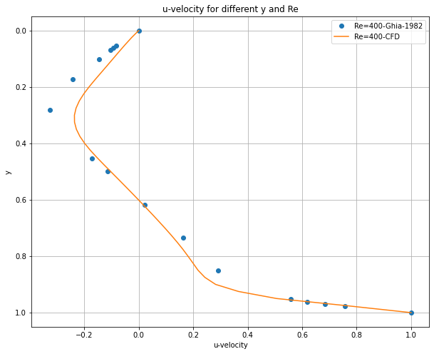
Benchmark using a reference data (Ghia-1982)#
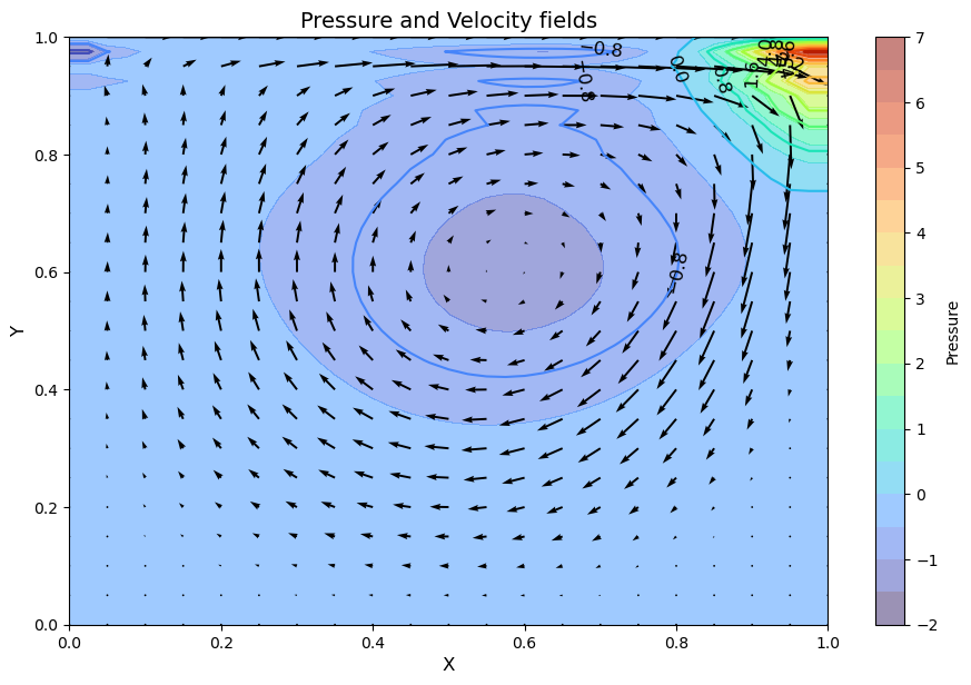
Try a case with Re = 400 and what happens?#
rho = 1
c= 4
nu = 0.01
dt = 0.001

u = np.zeros((ny,nx))
v = np.zeros((ny,nx))
p = np.zeros((ny,nx))
b = np.zeros((ny,nx))

print("Reynold's number =", c*length/nu)
Reynold's number = 400.0
nt = 10000

start_time = time.time()

u, v, p = cavity_flow(nt, u, v, dt, dx, dy, p, rho, nu)

end_time = time.time()
# Compute running time
running_time = end_time - start_time
print(f"Running time: {running_time} seconds")


# Create figure and set dpi and figure size
fig = plt.figure(figsize=(11,7), dpi=100)

# Contourf plot for pressure field with colorbar
cf = plt.contourf(X, Y, p, alpha=0.5, cmap='turbo', levels=20)
plt.colorbar(cf, label='Pressure')

# Contour plot for pressure field outlines
contour = plt.contour(X, Y, p, cmap='turbo', levels=10)
plt.clabel(contour, inline=False, fontsize=12, colors = 'black')

# Quiver plot for velocity field
quiv = plt.quiver(X[::2, ::2], Y[::2, ::2], u[::2, ::2], v[::2, ::2])

# Setting labels for the x and y axes
plt.xlabel('X', fontsize=12)
plt.ylabel('Y', fontsize=12)

# Setting the title for the plot
plt.title('Pressure and Velocity fields', fontsize=14)

# Display the plot
plt.show()
0%| | 0/10000 [00:00<?, ?it/s]
0%| | 8/10000 [00:00<02:15, 73.74it/s]
0%|▏ | 31/10000 [00:00<01:01, 162.02it/s]
2%|█▏ | 155/10000 [00:00<00:15, 643.32it/s]
3%|██▎ | 293/10000 [00:00<00:10, 927.89it/s]
4%|███▏ | 414/10000 [00:00<00:09, 1026.70it/s]
5%|████▏ | 536/10000 [00:00<00:08, 1091.47it/s]
7%|█████▎ | 690/10000 [00:00<00:07, 1235.97it/s]
11%|████████ | 1061/10000 [00:00<00:04, 2019.25it/s]
16%|███████████▉ | 1568/10000 [00:00<00:02, 2968.89it/s]
22%|████████████████▋ | 2195/10000 [00:01<00:01, 3984.80it/s]
29%|██████████████████████ | 2905/10000 [00:01<00:01, 4935.92it/s]
37%|███████████████████████████▉ | 3683/10000 [00:01<00:01, 5798.38it/s]
45%|█████████████████████████████████▉ | 4458/10000 [00:01<00:00, 6387.05it/s]
52%|███████████████████████████████████████▊ | 5234/10000 [00:01<00:00, 6799.37it/s]
60%|█████████████████████████████████████████████▋ | 6014/10000 [00:01<00:00, 7099.19it/s]
68%|███████████████████████████████████████████████████▍ | 6772/10000 [00:01<00:00, 7243.58it/s]
75%|█████████████████████████████████████████████████████████▎ | 7548/10000 [00:01<00:00, 7398.51it/s]
83%|███████████████████████████████████████████████████████████████▏ | 8322/10000 [00:01<00:00, 7498.90it/s]
91%|█████████████████████████████████████████████████████████████████████▏ | 9101/10000 [00:01<00:00, 7585.00it/s]
99%|███████████████████████████████████████████████████████████████████████████ | 9882/10000 [00:02<00:00, 7651.96it/s]
100%|███████████████████████████████████████████████████████████████████████████| 10000/10000 [00:02<00:00, 4929.40it/s]
l1norm_u =  4.480934823505844e-07 l1norm_v =  5.794213521550258e-07 l1norm_p =  5.24350596698032e-07
Running time: 2.053713321685791 seconds
import pandas as pd
import matplotlib.pyplot as plt

# Read the txt file
with open('Ghia-1982.txt', 'r') as file:
    lines = file.readlines()

# Adjust the lines range to match your data
lines = lines[5:-7]  # Adjust these numbers

# Process lines to obtain data
data = [list(map(float, line.split())) for line in lines]

# Create DataFrame from data
df = pd.DataFrame(data, columns=['y', 'Re=100', 'Re=400', 'Re=1000', 'Re=3200', 'Re=5000', 'Re=7500', 'Re=10000'])

# Set y as index
df.set_index('y', inplace=True)

# Plotting
# plt.figure(figsize=(10,8))
# for column in df.columns:
#     plt.plot(df[column].values, df.index.values, label=column) # use .values to get numpy arrays

# plt.xlabel('u-velocity')
# plt.ylabel('y')
# plt.title('u-velocity for different y and Re')
# plt.legend()
# plt.gca().invert_yaxis()  # To invert y-axis
# plt.grid(True)
# plt.show()
# Plotting
plt.figure(figsize=(10,8))

plt.plot(df['Re=400'].values, df.index.values, 'o', label='Re=400-Ghia-1982') # use .values to get numpy arrays
plt.plot(u[:,int(ny/2)]/c, y, label='Re=400-CFD') #

plt.xlabel('u-velocity')
plt.ylabel('y')
plt.title('u-velocity for different y and Re')
plt.legend()
plt.gca().invert_yaxis()  # To invert y-axis
plt.grid(True)
plt.show()
Try a case with Re = 1000 and what happens?#
For a side-by-side efficiency comparison between Chorin’s projection and the direct coupling method, we’ve replicated the direct coupling approach and executed it below.
def cavity_flow_direct(nt, u, v, dt, dx, dy, p, rho, nu):

    def build_up_b(b, rho, dt, u, v, dx, dy):

        b[1:-1, 1:-1] = (rho * (1 / dt *
                        ((u[1:-1, 2:] - u[1:-1, 0:-2]) /
                         (2 * dx) + (v[2:, 1:-1] - v[0:-2, 1:-1]) / (2 * dy)) -
                        ((u[1:-1, 2:] - u[1:-1, 0:-2]) / (2 * dx))**2 -
                          2 * ((u[2:, 1:-1] - u[0:-2, 1:-1]) / (2 * dy) *
                               (v[1:-1, 2:] - v[1:-1, 0:-2]) / (2 * dx))-
                              ((v[2:, 1:-1] - v[0:-2, 1:-1]) / (2 * dy))**2))


        return b

    # This is another version of pressure_poisson function with l1norm_target
    def pressure_poisson_l1norm(p, dx, dy, b, l1norm_target):
        pn = np.empty_like(p)
        pn = p.copy()

        l1norm = 1
        small = 1e-8
        niter = 0
        while l1norm > l1norm_target:
            niter += 1   # count the number of iterations for convergence
            pn = p.copy()
            p[1:-1, 1:-1] = (((pn[1:-1, 2:] + pn[1:-1, 0:-2]) * dy**2 +
                              (pn[2:, 1:-1] + pn[0:-2, 1:-1]) * dx**2) /
                              (2 * (dx**2 + dy**2)) -
                              dx**2 * dy**2 / (2 * (dx**2 + dy**2)) *
                              b[1:-1,1:-1])

            p[:, -1] = p[:, -2] # dp/dx = 0 at x = 2
            p[0, :] = p[1, :]   # dp/dy = 0 at y = 0
            p[:, 0] = p[:, 1]   # dp/dx = 0 at x = 0
            p[-1, :] = 0        # p = 0 at y = 2
            l1norm = (np.sum(np.abs(p[:]-pn[:])) / (np.sum(np.abs(pn[:]))+small))

        return p, niter

    def velocity_u_update(u, dx, dy, dt, rho, p, un, vn):

        u[1:-1, 1:-1] = (un[1:-1, 1:-1]-
                        un[1:-1, 1:-1] * dt / dx *
                        (un[1:-1, 1:-1] - un[1:-1, 0:-2]) -
                        vn[1:-1, 1:-1] * dt / dy *
                        (un[1:-1, 1:-1] - un[0:-2, 1:-1]) -
                        dt / (2 * rho * dx) * (p[1:-1, 2:] - p[1:-1, 0:-2]) +
                        nu * (dt / dx**2 *
                        (un[1:-1, 2:] - 2 * un[1:-1, 1:-1] + un[1:-1, 0:-2]) +
                        dt / dy**2 *
                        (un[2:, 1:-1] - 2 * un[1:-1, 1:-1] + un[0:-2, 1:-1])))
        return u

    def velocity_v_update(v, dx, dy, dt, rho, p, un, vn):

        v[1:-1,1:-1] = (vn[1:-1, 1:-1] -
                        un[1:-1, 1:-1] * dt / dx *
                        (vn[1:-1, 1:-1] - vn[1:-1, 0:-2]) -
                        vn[1:-1, 1:-1] * dt / dy *
                        (vn[1:-1, 1:-1] - vn[0:-2, 1:-1]) -
                        dt / (2 * rho * dy) * (p[2:, 1:-1] - p[0:-2, 1:-1]) +
                        nu * (dt / dx**2 *
                        (vn[1:-1, 2:] - 2 * vn[1:-1, 1:-1] + vn[1:-1, 0:-2]) +
                        dt / dy**2 *
                        (vn[2:, 1:-1] - 2 * vn[1:-1, 1:-1] + vn[0:-2, 1:-1])))
        return v

    un = np.empty_like(u)
    vn = np.empty_like(v)
    pn = np.empty_like(p)
    b = np.zeros((ny, nx))
    small = 1e-8
    for n in tqdm(range(nt)):
        un = u.copy()
        vn = v.copy()
        pn = p.copy()
        b = build_up_b(b, rho, dt, u, v, dx, dy)
        #p = pressure_poisson(p, dx, dy, b)
        p, niter = pressure_poisson_l1norm(p, dx, dy, b, 1e-4)
        #print(niter)

        u = velocity_u_update(u, dx, dy, dt, rho, p, un, vn)
        v = velocity_v_update(v, dx, dy, dt, rho, p, un, vn)

        u[0, :]  = 0
        u[:, 0]  = 0
        u[:, -1] = 0
        u[-1, :] = c    # set velocity on cavity lid equal to c
        v[0, :]  = 0
        v[-1, :] = 0
        v[:, 0]  = 0
        v[:, -1] = 0

    l1norm_u = (np.sum(np.abs(u[:]-un[:])) / (np.sum(np.abs(un[:]))+small))
    l1norm_v = (np.sum(np.abs(v[:]-vn[:])) / (np.sum(np.abs(vn[:]))+small))
    l1norm_p = (np.sum(np.abs(p[:]-pn[:])) / (np.sum(np.abs(pn[:]))+small))
    print("l1norm_u = ",  l1norm_u, "l1norm_v = ",  l1norm_v, "l1norm_p = ",  l1norm_p)
    return u, v, p
u = np.zeros((ny, nx))
v = np.zeros((ny, nx))
p = np.zeros((ny, nx))
b = np.zeros((ny, nx))
nt = 10000
c = 1

start_time = time.time()

u, v, p = cavity_flow_direct(nt, u, v, dt, dx, dy, p, rho, nu)

end_time = time.time()
# Compute running time
running_time = end_time - start_time
print(f"Running time of the direct coupling: {running_time} seconds")

start_time = time.time()

u, v, p = cavity_flow(nt, u, v, dt, dx, dy, p, rho, nu)

end_time = time.time()
# Compute running time
running_time = end_time - start_time
print(f"Running time of the Chorin's projection: {running_time} seconds")
0%| | 0/10000 [00:00<?, ?it/s]
0%| | 8/10000 [00:00<02:09, 76.98it/s]
0%|▏ | 28/10000 [00:00<01:07, 147.41it/s]
2%|█▍ | 180/10000 [00:00<00:12, 764.13it/s]
4%|███▎ | 428/10000 [00:00<00:06, 1433.40it/s]
7%|█████▋ | 731/10000 [00:00<00:04, 2004.68it/s]
11%|████████▏ | 1073/10000 [00:00<00:03, 2482.32it/s]
16%|███████████▊ | 1557/10000 [00:00<00:02, 3248.98it/s]
21%|████████████████ | 2117/10000 [00:00<00:01, 3993.53it/s]
28%|█████████████████████ | 2764/10000 [00:00<00:01, 4764.08it/s]
34%|██████████████████████████ | 3436/10000 [00:01<00:01, 5364.96it/s]
41%|███████████████████████████████▏ | 4107/10000 [00:01<00:01, 5773.62it/s]
48%|████████████████████████████████████▎ | 4780/10000 [00:01<00:00, 6061.45it/s]
55%|█████████████████████████████████████████▍ | 5458/10000 [00:01<00:00, 6278.37it/s]
61%|██████████████████████████████████████████████▌ | 6126/10000 [00:01<00:00, 6397.99it/s]
68%|███████████████████████████████████████████████████▌ | 6792/10000 [00:01<00:00, 6474.42it/s]
74%|████████████████████████████████████████████████████████▌ | 7440/10000 [00:01<00:00, 6439.26it/s]
81%|█████████████████████████████████████████████████████████████▌ | 8095/10000 [00:01<00:00, 6472.02it/s]
88%|██████████████████████████████████████████████████████████████████▋ | 8768/10000 [00:01<00:00, 6548.52it/s]
94%|███████████████████████████████████████████████████████████████████████▌ | 9423/10000 [00:01<00:00, 6541.21it/s]
100%|███████████████████████████████████████████████████████████████████████████| 10000/10000 [00:02<00:00, 4996.88it/s]
0%| | 0/10000 [00:00<?, ?it/s]
1%|█ | 130/10000 [00:00<00:07, 1298.59it/s]
l1norm_u =  2.0964336749894792e-06 l1norm_v =  2.8019156614369277e-06 l1norm_p =  2.349586199251818e-06
Running time of the direct coupling: 2.0026907920837402 seconds
8%|██████▌ | 845/10000 [00:00<00:01, 4722.32it/s]
16%|████████████ | 1593/10000 [00:00<00:01, 5976.87it/s]
23%|█████████████████▊ | 2339/10000 [00:00<00:01, 6559.48it/s]
30%|███████████████████████▏ | 3047/10000 [00:00<00:01, 6744.33it/s]
38%|████████████████████████████▊ | 3783/10000 [00:00<00:00, 6951.51it/s]
45%|██████████████████████████████████▍ | 4525/10000 [00:00<00:00, 7103.77it/s]
53%|████████████████████████████████████████ | 5270/10000 [00:00<00:00, 7212.08it/s]
60%|█████████████████████████████████████████████▋ | 6008/10000 [00:00<00:00, 7261.94it/s]
67%|███████████████████████████████████████████████████▎ | 6746/10000 [00:01<00:00, 7298.16it/s]
75%|████████████████████████████████████████████████████████▉ | 7489/10000 [00:01<00:00, 7336.85it/s]
82%|██████████████████████████████████████████████████████████████▍ | 8223/10000 [00:01<00:00, 7332.05it/s]
90%|████████████████████████████████████████████████████████████████████▏ | 8966/10000 [00:01<00:00, 7360.63it/s]
97%|█████████████████████████████████████████████████████████████████████████▊ | 9713/10000 [00:01<00:00, 7392.05it/s]
100%|███████████████████████████████████████████████████████████████████████████| 10000/10000 [00:01<00:00, 6930.98it/s]
l1norm_u =  9.146630711997816e-08 l1norm_v =  1.2481511707631306e-07 l1norm_p =  8.195025302473762e-08
Running time of the Chorin's projection: 1.4441249370574951 seconds
Chorin’s projection is more efficient than the direct coupling approach!